Evaluating the Performance of Convolutional Neural Network Based xG Models

Charles William · July 15, 2020

xG   Machine Learning   Models

• An xG model built using only tracking data freeze frames is demonstrated, producing encouraging results compared to a current state-of-art model

• Using spatial pattern recognition this model makes an attempt to learn the underlying relationship between the situation a shot was taken and probability of a goal being scored

• This leads to the possibility of improved extrapolation of rare events and fewer training samples required for a high quality model compared to decision tree based solutions widely used

• High quality xG models can be produced in workflows where no event data is available but footage exists, such as in lower division matches and training sessions - the latter being of particularly high value

Background and Motivation

Many of the more common metrics produced by football data providers today, including xG, make use of a machine learning classifier model variety called decision trees. A decision tree takes input observations from the environment and uses them to learn the best sets of criteria for these values that can predict an output variable. The training process tries out different values and combinations of input variables and criteria until it settles on the tree that minimises a chosen error value. Model performance is then evaluated by comparing the model predictions to the true output using data it hasn’t seen before.

The figure below shows a highly simplified decision tree that could be used for an xG model, albeit a very poor one. The input variables used make up nodes and the criteria for these nodes make up the branches. The model estimate is found at the last node of a branch. So here we have play type, distance from goal, and attack type when a shot was taken as input variables and some criteria that can be used to estimate the probability of a goal.

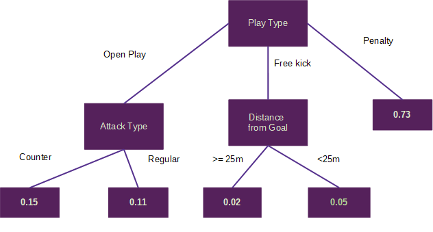
A basic example of a decision tree which could be used as an xG model. The node and branch values are derived from a training process, with xG values for new shots being derived by following the applicable path down the tree

Of course in the real world the trees developed would be far more complex with far more meaningful inputs. Many top end models take advantage of the benefits of combining hundreds or thousands of them to get more accurate results in what is known as an ensemble.

StatsBomb’s xG model, Goalkeeper evaluation framework, passing uniqueness model, and KU Leuven’s VAEP* action value - all use forms of decision tree model. The results of these models speak for themselves, with the authors of all of these examples taking validation seriously. As such, all have published various model quality metrics alongside their methods.

There are however two key, inherently linked disadvantages to the decision tree based approach. Firstly, tree based models are bad at dealing with outliers, rare or extreme events. Tree models do not extrapolate well, so if the model hasn’t seen an input before or only has a handful of samples it deems relevant to draw upon it will likely give a poor quality prediction. This leads to the second issue which is that to ensure that all input scenarios, including rare ones, have good representation when training, a very large amount of data is required.

This study takes a look at an alternative modelling method, using the case of xG as an experiment: Convolutional Neural Networks, or CNNs.

CNNs are a type of neural network that look for patterns or distinct objects in image data and use them to make classifications. Digitising handwritten letters or picking out a cat in photo are situations where a CNN could be used. The background won’t be dwelled upon here, but a very good introduction to CNNs can be found on Ujjwal Karn’s data science blog.

One of the key properties of CNNs is that they attempt to learn spatial patterns in data. That means that rather than infer a given spatial relationship in the data at every point in space, a top-level pattern that may occur at different locations can be identified. In the case of an xG model it would be advantageous for the model to recognise that a group of defenders directly in front of the ball is bad for scoring prospects no matter where that situation occurs on the pitch.

Another advantage is that a CNN attempts to model the underlying process that is mapping the input data to the xG value. So any new value that is present to model gets transformed through the same function. This is in contrast to a decision tree based model which uses a “nearest neighbours” approach to group shots it thinks are similar together. When a new value which the model hasn’t encountered before is presented it will often struggle to produce a quality output as it has no reference point. To combat this, decision tree based xG models might be trained on huge datasets to minimise the chance of unseen new data appearing, potentially sacrificing time and scope relevancy.

In addition to aiming to reduce training data sample size and improve handling of rare cases, there are some practical motivations to developing CNN models in football data analysis. Traditional high-end xG models are trained on a multitude of features that originate from event data. Event data can be expensive to obtain from a commercial vendor where it exists, or if it doesn’t exist e.g. for lower league matches or training sessions it can be both expensive and time consuming to produce independently.

The ability to generate high quality models directly from video footage is therefore an attractive proposition to analysts. Auto-coding of tracking data from video via computer vision (CV) is a considerably easier problem to solve than generating high quality event data from the same method. For the former, “only” object tracking, pitch mapping, and cleaning are required. Technology such as this that is also able to infer body orientation of players has also been demonstrated. The latter requires this plus a whole host of different algorithms to infer action types and situations based on video frames, with comparable performance to human performance a long way from being demonstrated to the best of the author’s knowledge.

In the case of developing models for use on training session analysis CV techniques may not even be required, as all players could be wearing GPS receivers from which a tracking data set could be readily produced.

This study aims to investigate if an xG model of comparable performance to a state-of-the-art commercial offering could be developed using only a tracking data snapshot from the moment the shot was taken utilising a CNN based approach. Due to the shortcomings of data available to train the model (which will be discussed in the next section) it is hoped this study will provide a proof of concept as opposed to a deployable production model.

*In the paper the team talk about moving towards a Generalized Additive Model (GAM) approach for increased interpretability.

Methodology

For our model we will try to infer the probability of a goal being scored based only on the location of players at the time when shot was taken, which can be interpreted as xG. This location data will be taken from “freeze frames” provided as part of StatsBomb’s open data set which consisted of around 21,000 shots at the time of writing. The strength of this approach is that a large amount of the information required to create a high quality xG model is contained within this tracking data freeze frame, including:

• The location of the shot

• The location of the goalkeeper

• The location of defenders between the ball and the goal

From this the model can theoretically infer the angle and distance of the shot, how much pressure the shooter is under by defenders, if there was an open goal, and other factors.

That said, this data doesn’t contain everything we might need. Factors that are missing that have been shown to contribute include:

• Body part shot was taken from

• Height the shot originated from

Plus there is other information missing that one might instinctively think is a factor such as body orientation and whether the shot was taken first time. We’ll see how much the omission of these factors affects the model quality, but focusing on what we do have, we can move on to some data pre-processing.

It is important to re-state that the aim of this wasn’t to provide a final working solution since data availability is a constraint, but more of a proof of concept. To that end we will prune the data available to help us get started while also taking a few liberties that we would never do with a production model:

• We are going to use all shots available in the StatsBomb open data set, so around 21,000 as a starting point. Around 1/3 of this data is from Barcelona games featuring Lionel Messi, another 1/3 is from women’s data, and the final 1/3 is an assortment of men’s Champions League finals, a men’s Word Cup, and the Arsenal Invincibles from 2003/04. The reason these distinct subsets are being combined is that it is estimated that at least that order of magnitude for number of shots will be needed to get a reasonable result. This is of course highly problematic since training using data influenced from just one team, mixing data from men’s and women’s football, and using data from 16-17 years ago are all bad ideas for developing a well defined, time relevant model.

• We are going to strip out headers. This has been done to give the model a fair chance with the data we have, given a header is highly distinctive shooting situation. To be a truly event-less input we would have to be able to generate an xG for these shots as well without categorising as a header/ no header. It is speculated that by using multiple frames of tracking data you would be able to infer a significant amount of this information, so this is by no means a show-stopper. For this proof of concept, given we only have a single frame, the author is comfortable stripping headers out.

• We are going to use only shots that are taken within 40 standardised units (Statsbomb’s equivalent to yards) on the x axis to goal, leaving an 80 x 40 pitch coverage area. This captures the vast majority of shots, whilst maintaining a reasonable model size whilst also allowing us to perform standard CNN operations.

• We are going to use location data coordinates rounded to the nearest integer. It is with deep regret that we’ll be throwing away StatsBomb’s 0.1m resolution location data for many shots. This is only so we have a manageable model size to start with. There is no conceptual problem with using 0.1m resolution data, it is just there is a limited amount of computational resources available so steps were needed to make the model as easy to train as possible without sacrificing the integrity of the study.

To get the data into a state that a CNN can both recognise and derive useful patterns and relationships we have to perform some further pre-processing. The processing scheme that we will use will turn a freeze frame into 3 separate binary images, or channels.

Channel 0 will contain the ball location data, channel 1 will contain the goalkeeper location data, and channel 2 will contain the defender location data. We could add a fourth channel, containing teammate location data but a model complexity-accuracy trade off decision has been made to omit it in this first attempt at developing the model as StatsBomb’s research showed that attackers behind ball is around half as important as a variable than defenders behind ball. We are of course losing some useful information about bodies between the ball and the goal, but we’ll see where we get to without.

The input of the model will therefore be 3 channels or 80x40 binary images, and from these we will attempt predict whether this input, representing a shot freeze frame, resulted in a goal. The model output will be a value between 0 and 1, where 0 represents no goal and 1 represents a goal. We have to be careful when interpreting what this output is actually telling us, but a reasonable interpretation is that this value is an index of confidence in the classification. So for example an output of 0.9 suggests high confidence the shot will result in a goal, and an output of 0.1 suggests low confidence.

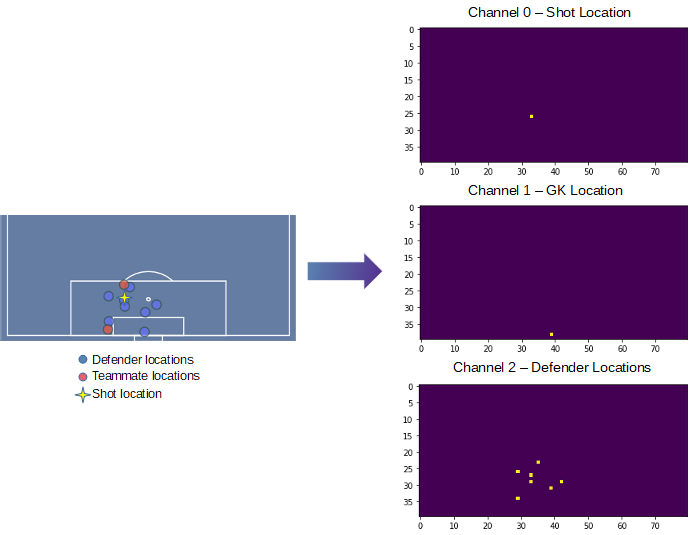
Freeze frames represented as three binary image channels. Teammate locations have been stripped out of the frame for processing

We then have a very important final validation step to ensure that this index of confidence is actually representative of the probability of a goal outcome given the input data, which we can call xG, as this is by no means guaranteed for many standard machine learning techniques.

It is often said, with good reason, that there is little point in developing a CNN from scratch these days. This is because some of the most highly-performing, state-of-the-art architectures are free to use, open sourced, and have a wealth of high quality documentation. In addition, they are all highly optimised and extremely flexible on a wide range of tasks. Well known examples include ResNet, Inception, DenseNet, and Xception, and these are often included in out of the box machine learning libraries such as Keras.

For this study conventional wisdom will be ignored, partly because using something like ResNet on primitive binary images seems a bit overkill, but also there is an opportunity to learn about CNNs and practical considerations for this application, namely predictive modelling in football for which not much literature exists.

Given we’re predicting whether the shot results in a goal or not, this is a binary classification task. We’ll use a sigmoid activation function on the last layer to constrain our output to 0-1, and binary cross-entropy - equivalent to log loss in this single class case - as our loss function.

An attractive feature of log loss is that it will punish predictions that are made with a high level of confidence that turn out to be wrong, rather than just noting the prediction was wrong. So for example if an iteration of the model predicted an xG value of 0.02 i.e. the model is very confident that this shot did not result in a goal, but the shot actually resulted in a goal, then the resulting log loss will be high and as such the model will try to correct itself for the next iteration.

Before we start building and training models we should take a moment to get a handle on what kind of performance, in terms of log loss, would represent a model that was working and actually learning interesting things. So let’s do some benchmarking.

The extremely useful sklearn library in Python has an easy to use one-line function that can calculate log loss given a set of predictions and a set of actual outcomes. To benchmark the CNN model we will compare typical log loss values seen with different model types.

The model types chosen are:

• A random number generator

• A model that predicts the average xG of the training set for all shots

• A logistic regression that uses shot x,y location only as inputs

• StatsBomb’s xG model

Even though we’ll be setting aside thousands of shots for testing i.e. the model won’t have access to these shots when training, to make sure the comparison is fair we’ll use exactly the same set of shots to evaluate each of these models and the CNN, so a constant random seed will be set for the duration of the experimentation.

Since we are starting from scratch it makes sense to start simple when it comes to architecture. We want the model to be as simple as possible whilst having enough complexity to capture the relationship between the ball location, player locations, and xG.

The first model will be pretty much as standard as they come. It was assumed that the model would be learning a reasonably complex representation so 3 convolution layers and a single dense layer were chosen as a baseline. The convolution layers will be doing all the looking for patterns within the binary images to create spatial representations and the dense layer will then select appropriate combinations and weightings of these representations to produce a classification estimate.

The first model has a 32 – 64 – 128 3x3 convolution structure with a 32 node dense layer. Between each convolution layer we have a 2x2 max pooling layer. We’re using a vanilla SGD optimiser and batch size of 32. We will train the model on 12,600 shots and test it on 5,400 unseen shots. All work will be carried out in Python using the Keras API wrapper around Tensorflow.

Results, Optimisation and Discussion

After 88 epochs the training process completes and reverts all model parameters back to the best result it found when trying to minimise log loss. On the whole the training process looked encouraging. It was definitely learning something as the training loss was steadily decreasing from its initial state, and the validation loss, that is the loss on data the model hasn’t seen, was also decreasing as the epochs progressed.

Some things that were pleasing to have avoided straight off were the model not training at all, rapid over-fitting of training data, and general nonsense output values. The model’s best result on the test set during training was a log loss of 0.2938. But what does that mean? Is that good?

Let’s now re-visit our benchmark models and see how they perform on the exact same data.

• Random Number Generator - 0.9985

• Fixed average xG of the training set (0.1144) - 0.3662

• x,y shot location logistic regression - 0.3298

• StatsBomb xG - 0.2813

As a bonus we can also generate a ballpark figure for how a perfect probability prediction model would perform. If a model predicted the correct output , 0 or 1, for every shot the log loss would be zero. But we’re modelling a stochastic process and so we can ask what would the log loss on this test set be if the model gave the exactly correct probability of a goal being scored for each shot?

We don’t know what the true probability of scoring for each shot was, but let’s assume the StatsBomb model output is the ground truth. We can be relatively confident that the true goal probability distribution broadly matches the StatsBomb model’s xG distribution for the shot set. So plugging the xG values in as our prediction, and then running a simulation of the 0,1 outcomes of these shots and using this as the actual output, we get a log loss of 0.2675.

The CNN has exceeded initial expectations for this first attempt. Log loss is much closer to the StatsBomb model than the location based logistic regression. But log loss is not the whole story for evaluating the quality of this model.

As touched upon earlier, the output of our model is in effect an index of confidence that the shot resulted in a goal or not. We don’t actually know yet if this can be reasonably interpreted as an xG probability. We need to inspect what is known as the calibration curve, also known as a reliability diagram.

Here we compare the output of our model which we are claiming to represent xG, with the actual goal probability of the shots in our test set. Now of course, we don’t actually know what the true goal probability of each shot was. What we can do instead is to split our predictions into bins based on predicted xG value, and then compare the average xG value of the bin with the average goals per shot value from those same shots. Ideally this plot will be a diagonal line going from (0,0) to (1,1), showing matching between predicted probability and goal outcome proportion.

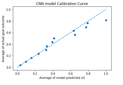
This is again another encouraging result. We can see good matching up to xG values of around 0.35 and then some error starts to creep in. Part of this is undoubtedly an issue with the model, as we know there is improvement to be had in terms of log loss, however we know that the number of shots at a given xG decreases as the xG value increases, so we would expect the calibration curve to be a bit noisier at the higher xG values.

Let’s now turn our attention to trying to improve the model by experimenting with different architectures, layer types, and optimisation functions.

With so many model parameters, or hyperparameters, to tune in attempt to improve model performance. It can be difficult to know where to begin. Fortunately hyperparameter tuning tools are available that wrap around Keras, meaning the process becomes a lot simpler to get started at least. I’ve used the module keras tuner here.

After providing the tuner function with a parameter space to search for optimisations including filters for each convolution layer, kernel size for each layer, and number of nodes in the dense layer the following architecture was returned as optimal:

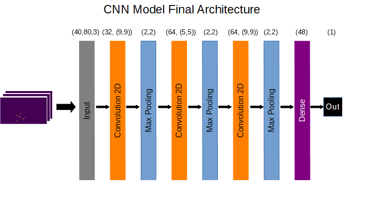
Further experimentation resulted in replacing the standard ReLU activation function with a “leaky” version. Negative values input to this function now have a small negative slope rather than being hard clipped to zero. This function is highly effective in allowing the network to represent non-linear functions with minimal computation, which is what we want, but comes at the cost of introducing saturation to zero when large negative values are input during training. This leaky version gives activations that have saturated to zero, and hence play no role in differentiating between input values, a chance to recover during training with a small gradient.

The final model achieved a log loss of 0.2909 and produced the following calibration curve, shown along side the StatsBomb model on the same data:

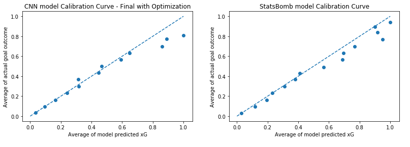
Further investigation with 2 layer and 4 layer architectures yielded log loss values of 0.2951 and 0.2933 respectively, with calibration curves showing larger mis-calibration at higher xG values compared to the 3 layer architecture.

The final question we will look to address is how much training data is actually needed to achieve a high quality result. After all, one of the project aims was to build a pathway towards high quality models that require less training data than their decision tree based counterparts.

Running the training process from scratch with training sets of different sizes yielded the following results:

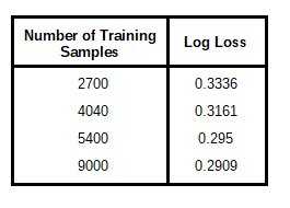
It was observed that a log loss value and calibration curve that was visually comparable to the optimised model trained on 12,600 shots was achieved when approximately 9,000 shots were used. At lesser values, there was considerable log loss drop off and noticeable deficiencies in the calibration curve outputs.

Post-calibration

A noticeable trait of the calibration curve is a flattening below the 1:1 line where the model is predicting xG > 0.8. The average of the true probability of these shots is inferred to be significantly lower than predicted, suggesting some sort of systemic failure could be occurring rather than noise.

This kind of thing is expected for all different kinds of machine learning models of varying complexity. It is why inspecting the calibration curve is so important. There are techniques available that can correct for these kinds of model error. Here we will attempt one – isotonic regression.

What we will be doing is essentially machine learning on top of machine learning. We will learn the CNN model representation, than we will learn a transform that can be applied to the output of this model to “straighten” the calibration curve and hopefully reduce log loss.

To do this we need to retrain the model but split the data into a three sets now: a CNN model training set, a isotonic regression training set, and a final test set. We use this additional training set to decouple the correction training from the original model training – otherwise we risk overfitting to the training data. We also can’t use the test set as the isotonic regression will learn the transformation of the test set only and will not be robust to new data.

One interesting thing to note is with the new train and test split the CNN model now achieves a log loss of 0.2878. Nothing about the model has changed, it has just been presented with different, and indeed less, test data. This suggests it has got lucky and has been given a test set it finds easier to predict. The other interesting point is the StatsBomb model’s loss is now only 0.001 lower than the CNN. Further evidence that we are on the right track.

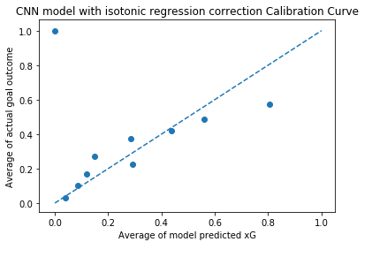
On inspection of the isotonic regression training set the calibration curve is pretty much the straight diagonal we were looking for. However the calibration curve of the test set is shown below – a clear abject failure. Log loss has become 0.2933, which although worse than before is still decent, but the calibration curve is all over the place. This output is not representative of an xG probability value.

Conclusion

The core aim of this study was to assess the feasibility of producing a xG model that was comparable in quality to leading decision tree models. Due to the limitations in data available for training it was unrealistic to expect a production ready model as the final result, and given the absence of temporal and z-axis derived features (such as a first time shot boolean or shot height categorical) the model was always destined to be sub-optimal.

However, the results obtained are encouraging for developing a pathway towards:

• Efficient use of data for time and scope focused model training – taking advantage of spatial patterns and handling unseen events acceptably.

• Development of non-event based models for applications where event coding is not possible or financially viable – perhaps taking advantage of Computer Vision technology to obtain relevant frames from video footage or using readily available GPS data.

With log loss performance well in advance of a location based logistic regression and close to (and almost identical to with some test set permutations) the StatsBomb decision tree model, in addition to a visually comparable calibration curve, this CNN approach has shown considerable potential.

It should be noted that the StatsBomb model is at a slight disadvantage when being compared to this model. The StatsBomb model was trained on a general shot set that is representative of a wider population, whereas the CNN model was trained on the unusual mixture of data from which test samples have been taken from as well. So the CNN model had the opportunity to learn the characteristics of the strange distribution that was generating the test data which the StatsBomb model did not. It is not entirely clear the magnitude of this disadvantage, however it is assumed to be not insignificant.

The noticeable weakness of the CNN model is the susceptibility to output a maximum predicted probability significantly below 1. This is not an issue unique to this model, as overly conservative predictions are a trait of many machine learning methods. It is unfortunate the attempt at post-calibration did not seem to work. With more, higher quality data and an alternative method such as Platt scaling, perhaps the results would be different.

Another often stated weakness of neural networks in general is the “black box” nature of the models that are produced. Whilst historically perhaps less effort was made to understand how a model had come to a decision about assigning a class prediction, this is certainly not the case today, with a number of dedicated tools and methods available to do just that. This primer from Stanford University is excellent in that regard.

However, even if you can see why a CNN made a certain decision, it doesn’t mean this “reasoning” will necessarily make sense to a human observer. In the below image we have a sample of input arrays for channel 2 - the opposition defenders channel - that would maximise the activation for filters in the third convolutional layer. These images are essentially what the model is looking for when trying to identify patterns that will help it make a decision. In the third convolutional layer there are 64 filters and as such 64 associated maximum activation inputs. 6 of these 64 are shown.​

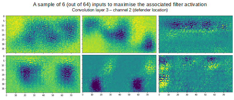
There are no easily interpretable features from this sample of input images that one might think are relevant when relating defender location to xG value. Yet, the model is able to provide a pretty good estimate of this value by searching for patterns such as these. This emphasises the point that although machine learning techniques such as this appear to be developing an understanding of the systems they are trying to model, this understanding falls far short of something that could be described as human-level understanding.

Possible next steps for this study would be to:

• Obtain a higher quality training set of freeze frame data – perhaps 2 consecutive seasons from the same league.

• Bring back headed shots into the set and add body part, shot starting height, body orientation, and a first time shot flag as inputs (these would be added as inputs to the dense layer, after the convolution layers) to ascertain their effect on model performance. Are these needed (violating our non-event data requirement) or can they be omitted without performance penalty?

• Obtain a tracking data set and use n frames prior to the shot to add temporal information to the model. It is not clear whether it would be best to include this as additional channels, an additional dimension, or indeed a different architecture such as an LSTM or other RNN.

• Make the model robust to frame area so all shots, even those taken from the half way line can be included.

• Develop a method for making use of 0.1m resolution without exploding model complexity.

• Incorporate a rotation invariant convolution filters for much more efficient pattern recognition such as https://ieeexplore.ieee.org/abstract/document/7560644

Acknowledgements

This work has been made possible due to the generosity of StatsBomb and their open data initiative.

Share: Twitter, Facebook