-
Attempting to quantify the value of a wide range of player actions using only event data has gained traction recently, with VAEP, xT, g+, and PV some of the most well known models.
-
All of these models return a single point estimate of “value” which seems sub-optimal given we know so much vital information hasn’t been considered by the model.
-
We also have no way of knowing how much trust we can place on any conclusions we are drawing without making an attempt to quantify the uncertainty inherent in our models.
-
We can define two types of uncertainty, esoteric and aleatoric, and explore some techniques to add this information to our models. Established and new metrics can both advance from a solid theoretical grounding to something that can actually be used as part of a real-life decision making process.
It is fair to say that event based threat/possession/action value models are starting to gain traction in the analytics community. Metrics you may have encountered include xT, VAEP, g+, and PV. There are key differences between these different model types in both what they try to measure and how they go about it, but what they have in common is they all are trying to expand the concept of value in football modelling to beyond shots at goal. They all also face an uphill task in trying to quantify this value in a way that is genuinely meaningful to an analyst using event data alone.
In terms of the latter, we can attribute a substantial amount of this to the lack of information on the location of teammates and opponents that are only available with tracking data or freeze frames. It is this information that would allow a model to differentiate between an exquisite through ball and a hospital pass for example, which clearly have dramatically different values to the team in possession. Unfortunately an event only model has no chance to do so in many cases.
That said, we are still presented with numbers that represent value or threat as outputs of these models and others like them. How useful are they to an analyst? In truth we have no idea, because the uncertainty of these models has not been quantified.
In a real-life decision making processes providing the uncertainty of a model alongside headline outputs is essential, not optional. We can’t just use a model or metric as a means to back up pre-held beliefs, and cover our eyes when they go against them. Any model that we can produce is only of value if it is robust enough to challenge existing thinking, and without knowing model uncertainty we are simply unable to do that.
Of course it is unrealistic for any model to get things right all the time, but we want to give our model the opportunity to say “actually, I don’t know the answer”.
The issue of displaying model uncertainty alongside outputs is a longstanding one in public football analytics. You can use some relatively basic maths to do so with values that can be observed like mean pass completion % , or mean shots on target %. But what about situations where we can’t directly observe what we are measuring such as action value or even xG?
This article will take a look at two of the main types of uncertainty we see in models and how we can quantify them. We’ll use the general concept of valuing actions to apply these methods using both VAEP as a case study and a custom demonstrator metric built from scratch.
Before we start it is always a good idea to refer to some prior work in this area. While I haven’t seen estimates of uncertainty attached to the task of valuing actions, there are a number of previous works that have used Bayesian techniques to do so with xG and derivatives. These include:
Uncertainty in xG: Part 1 - Domenic Di Francesco
Quantifying Finishing Skill - Marek Kwiatkowski
A “Messi vs All” Analysis of the xG Metric - Anıl Cem Arslan et al
The Problem
Let’s now take a look at why model uncertainty is such a problem for action value models that only use event data.
Consider the figure below. We have 3 pass receiving actions for which a model will use to try to learn how to assign value to actions. We can immediately see that while the pass receipt location and origin are identical for each, the value of receiving the ball in these situations is markedly different. However, for a model using event data only, we only have access to that receipt and origin locations (plus perhaps some locations and action types of previous actions, and at best some situational labels about whether a counter is in progress or not for example). So as far as the model is concerned these 3 situations are identical.
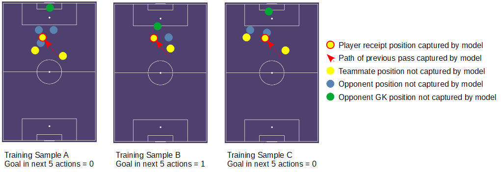
The consequence of this is the model will not be able to derive the true relationship between an action carried out in a given game state and value, with dramatically different true values being lumped into the same bucket from which it will draw conclusions. Our model will therefore output an average (it could be the arithmetic mean, mode, or a more sophisticated “hedge” to to try to minimise error dependent on the model architecture) of these differing situations, which could be largely meaningless in many situation and vary considerably compared to the true value of the situation.
We also need to consider how our model architecture will react to being so under-informed about the relationship it is trying to model. If you’re not telling a model about a key variable in a relationship between inputs and outputs, it is almost a given that it will behave differently depending on the data used to train it. It is clearly undesirable for a two models to value identical actions differently just because one was trained on games on a Saturday and the other was trained on games on a Wednesday night.
The amount of data we have is also a factor. If the sample of data we have to train a model isn’t large enough to be representative of the population we introduce further uncertainty.
This uncertainty attached to a lack of knowledge (not having player position data e.g. from tracking which we know intuitively is vital for understanding the value of an action) and/or lack of data is known as epistemic uncertainty. We can in theory reduce this uncertainty by adding more knowledge or data.
We also ideally would want to quantify the uncertainty that can be described along the lines of “anything can and does happen in football”. More formally, this is the uncertainty in the underlying data generating process. This uncertainty arises because the amount of value to a team, often measured in goals with common metrics of this type, differs significantly from seemingly identical situations. This might be due to particularly heroic or calamitous defending after a pass action as an example. A different source of uncertainty that falls under the same category is measurement noise. In this application you could imagine this noise stemming from the fat finger of an event feed coder.
These types of uncertainty are known as aleatoric uncertainty and can’t be reduced in practice.
This article outlines a relatively simple technique to incorporate epistemic uncertainty into a value action model using VAEP as a case study, and then a more complex method that quantifies both epistemic and aleatoric at the same time using a custom action value metric. Hopefully these examples will demonstrate both the importance of quantifying uncertainty and show the advantages that doing so brings to the analyst.
Elevating VAEP with Bagging
VAEP is a prominent model that has been developed in attempt to value a wide-ranging set of actions in addition to shooting that are carried out by players during a game. Such actions include passes, pass, receipts, interceptions, dibbles, and tackles. It was developed by Tom Decroos and colleagues, with the original paper available on arXiv. We are going to apply a technique called bootstrap aggregation, or “bagging”, to generate a confidence interval of sorts for VAEP and evaluate players from the 2019 FIFA Women’s World Cup.
A fundamental concept of bagging is we can use any model as a base, so we are not going to change anything in the VAEP implementation at all. As such we won’t delve into the specifics of the VAEP model, however check out this comparison of VAEP and another well known action valuation metric, xT, for everything you need to know.
The reason why we say confidence interval of sorts is that the term probably best describes what we will be doing despite not meeting formal mathematical criteria. VAEP returns a single number as an estimate for the value of an action which is essentially a mean value for all the possibilities that value could take. We’ll be taking a relatively large sample of those means as part of the bagging process to generate a distribution of sample means, which can loosely be defined as a bootstrap confidence interval.
This confidence interval is valuable as we can account for both sample size (e.g. if we were summing VAEP values for a player or team) and the fact that the model will be understanding the relationship between actions and value differently depending on the individual situation. For the latter case we may expect a model to interpret the value of a penalty state which is a largely fixed situation with more confidence than a pass reception 30 yards from goal, since the player receiving could have 10 players between them and the goal or be clean through. So quantifying this “understanding” gives the model a step-change in interpretability.
Let’s define the steps of how we generate this interval:
-
Define the base model
-
Take n samples of size p with replacement* of the training data, where n is typically >= 1000 and p is the size of the training data
-
Train the base model with each of the n samples, resulting in n models
-
Evaluate each of the n models with the inputs to be used for predictions, so you then have n predictions for each new input
-
Define e.g. the 2.5th and 97.5th percentiles for each prediction, or if aggregating by player/team/role for each set of predictions and the range becomes your confidence interval
For 1. we’re using vanilla VAEP, so not much more to add here. For 2. and 3. we’ll use StatsBomb’s FAWSL and NWSL open datasets to train the model which gives us around 560,000 actions, and we’ll sample with replacement 1000 times giving us 1000 models to train.
*This means we’ll pick values at random from our training set, but once a value is picked we’ll keep it in the set. We’ll do this until the sample size is as large as our original data So some values can and almost certainly will be picked more than once. We’ll then repeat this sampling process 1000 times. This is also known as bootstrap sampling.
For 4. we’ll use the Women’s World Cup set, giving us 1000 predictions of VAEP for each action in the set. We’ll then evaluate the distribution of those 1000 predictions to define our confidence interval for each value.
So what does it look like when evaluate the VAEP performance of players with this method?
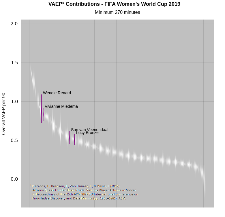
If we highlight some well known representatives from key roles we can see the model is more confident in the VAEP value for Lucy Bronze than it is for Wendie Renard. This also tells us Renard and Vivienne Miedema can be considered top performers by this metric even taking into account their worst-case values.
Let’s quickly look at the top 10 players in the above chart, and importantly, see who is at the top left, ruining the chart scaling in the process!
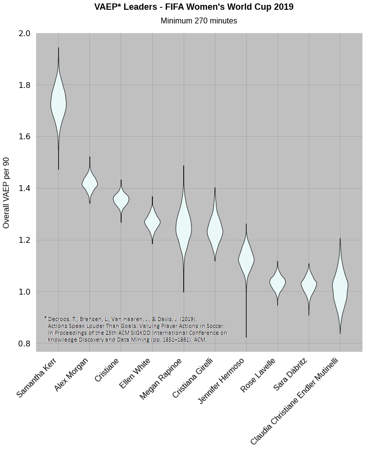
Perhaps no surprises there. Samantha Kerr’s lower bound is higher than everyone else’s upper bound with the exception of a tiny proportion of Alex Morgan’s distribution. We can safely say that VAEP thinks she had a good tournament.
We’ve now factored in esoteric uncertainty, that is uncertainty stemming from lack of knowledge and how that gets manifested with our model architecture, to the output values. This immediately adds vital information about model reliability that an analyst can use to give weight to their conclusions.
Completing the Picture with Full Probabilistic Modelling
Very little about the game of football can be said to be deterministic from the viewpoint of the observer. Without getting too philosophical, randomness plays a key role in pretty much everything we see on the pitch.
VAEP and related models such as g+, or xT are only able to output a single number representing value for a given input, which represents the typical value observed for situations that the model deems equivalent in the data it used to train. So we don’t actually have the actual value of the action that took place at all. For single point models such of this to have high quality, this “typical” value needs to be indistinguishable enough from the true value. Given we have so much key information missing when using event data only, this is definitely not the case for current public action value models.
If we say an action on average increases the probability of a goal in the next 5 events by 0.2, is that actually useful? Wouldn’t it be better to define what the actual change in probability actually was given the situation the player actually faced? Sounds nice in theory but we’ve said randomness is playing a key role in the outcome and we have the inherent uncertainty from the modelling process, so how can we define that with a single number? The truth is we can’t really.
Standard classification models output confidence scores that an input belongs to a class, which can be calibrated to the probability of class membership. Here classes could be e.g. this pass will lead to a goal / this pass will not lead to goal. So in these cases we actually do already have an output probability distribution which considers aleatoric uncertainty. But we are still sacrificing accuracy on one prediction so we can be more accurate on average over a larger set of actions. This is clearly sub-optimal.
So for binary or multi-category classification models we have quantified the aleatoric, or random noise, uncertainty associated with the mean value of an action for a given situation. By adding a bagging step we can quantify the esoteric, or lack of knowledge, uncertainty of that mean value. But we want to see the full distribution of all plausible values for that action given the information the model has, not just the mean, while also accounting for the information the model doesn’t have.
In addition, if we are fitting a regression model e.g. trying to predict the net xG from the next 5 events, we go back to having no probabilistic information at all and hence no aleatoric uncertainty consideration.
There are number of proposals to solve this out there in the wider world of data science and machine learning, but one such method that seems appealing is Mixture Density Networks. I’m in the middle of a full technical write-up (for transparency purposes mainly) of the work I have carried out in this area, so explanation of methodology and architecture of the model proposed will be kept brief here.
Work by Choi et al. demonstrated that MDNs capture both aleatoric and esoteric uncertainty. So it looks like this method is suitable to do what we want, although we may not be able to break down the magnitude of uncertainty by where they originate from. But that is probably of little concern to the end-user anyway.
Essentially instead of telling our model to predict a single number that represents the value of an action or game state, we tell it predict the parameters of a probability distribution which represent this value instead. In an ideal world this value would be normally distributed, so we would just predict a mean and standard deviation for each value. However, we don’t know what shape the distribution will have and it seems plausible it will vary from action to action.
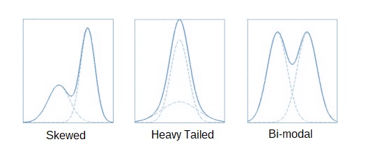
By representing action or state value as a mixture of several normal distributions, we have the flexibility to define a good approximation of a variety of different distribution shapes as the figure below shows. The number of normal distributions that make up the mixture, known as components, needs to be selected maximise the flexibility of the distribution shapes possible whilst minimising the model complexity.
The basic premise of the model is as follows: We will look to evaluate the value of non-shot, in-possession actions. That means for every pass, clearance, and take-on attempt we will output a state value distribution which represents the distribution of the net number of goals expected to be scored/conceded within the next 10 actions at the point the action was taken. We’re counting all distinct on-ball actions only, so for example when looking at past actions, a duel counts a 1 action event though there is one event per player involved.
We’ll then assign a value for the state at the point of the next pass, clearance, take-on, OR shot in the game event sequence.
The difference between these two state values will be deemed the action value. Essentially, how much did the number of expected goals in the next 10 events change as a result of the action.
Where the team in possession changes as a result of the action, the state value for the post-action state is the value of state for the opponent multiplied by -1. This allows us to factor in the cost of misplacing a pass or getting dispossessed as a result of a take-on attempt for example.
We’ll use 16 values including pitch location, binary flags concerning what type of action occurred, which team was in possession and time elapsed since the previous action over 10 previous actions for a state as one input. We’ll use 1D convolution to try and extract information about how the sequences of previous actions relate to state value. The hope is here that we can squeeze as much information about game context from this information when assigning value to a game state. We’ll then use 4 more values including pitch location, who is in possession, and whether it is a set piece, which give us information about the current state prior to the action.
We’ll tell the model to output mean and standard deviation parameters for a mixture of 4 normal distributions, as well as a proportion for each sub-distribution which will sum to 1.
The model looks like this:
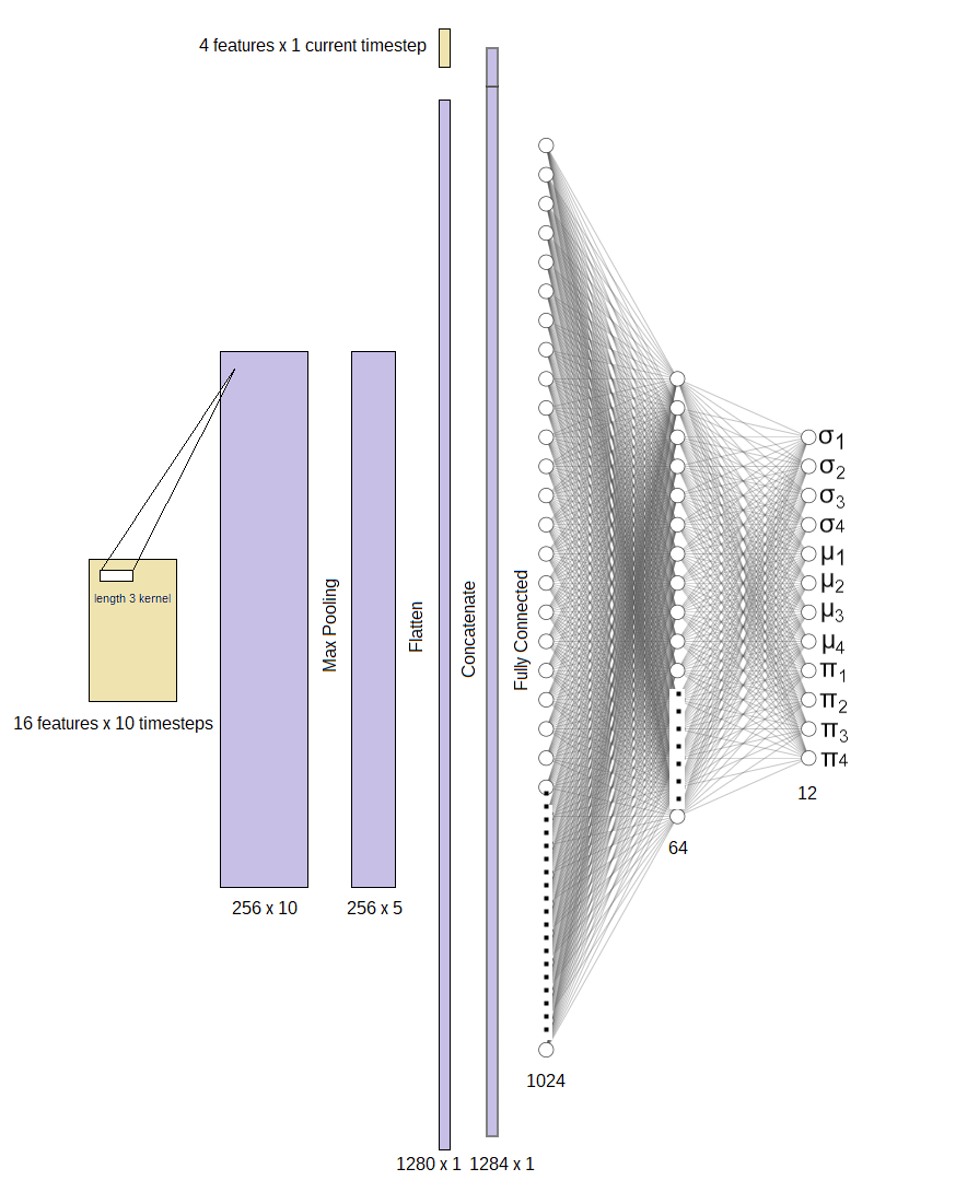
We’ll train it on net xG (i.e if a shot was conceded as a result of an action the value will be negative) produced from the following 10 actions from the state being predicted. We can then generate an “action value” by finding the difference between post and pre action state distributions.
One complication here is that these two distributions aren’t independent of each other, that is we would expect there to be some link between the value of these two consecutive states. If the pre-action state was in the middle of a dangerous counter, the post-action state has a reasonable, albeit not guaranteed chance of being within this same wider game situation. It is probably worth reiterating here how technical details such as how this is factored in are explained in detail in the full write-up.
Now for the interesting part – what do we get out of this when we value actions using this approach, and importantly, what additional benefit does it give an analyst?
Let’s plug in data from the Premier League 19/20 season and produce some probabilistic versions of some standard plots we’re used to seeing and some less common types that lend themselves to this new level of information we have.
Single Action
We’re used to seeing the value of an action represented as a single number, which as discussed is sub-optimal when so much key information is missing in the model and there is a significant level of randomness attached to the outcome. We can now produce a value distribution for every action.

This pass by Raúl Jiménez has a value anywhere from -0.05 to 0.15 goals added based on what we told the model. We can see that this pass put Adama Traoré clean through on goal, but of course the model doesn’t know that as it doesn’t have player positional data. We could also inspect the pre-action state value to see how valuable the situation was at the moment Jiménez played the pass – did he add the majority of value with this action or did the model think the situation was likely to be highly valuable already?
Value Creators
Moving on the staple of football analytics Twitter: the scatterplot. If we take a plot derived from single point estimates of value (by taking the mean of the distributions) we can produce something along the lines of this:
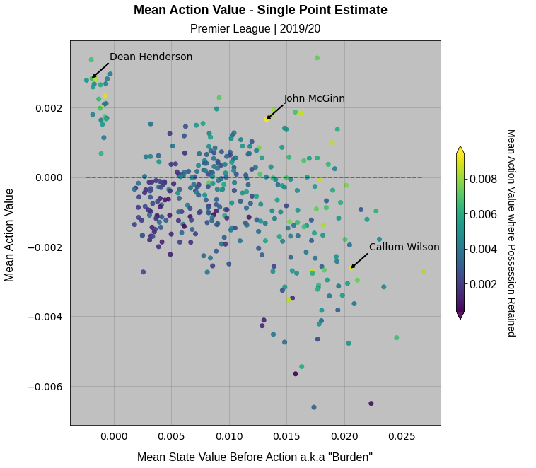
Here we’re looking for the value per action of players vs the value they started with pre-action, a term American Soccer Analysis has coined “burden” which I’m happy to borrow here for consistency. We have a goalkeeper cluster in the top left who all on average seem to add value, but of course playing so deep they have virtually no offensive value to lose when they give the ball away.
Contrast this with attacking players who largely reside in the bottom right of the plot, who typically receive the ball in valuable areas, who struggle to add value with non-shot actions. An additional layer we can add is the value per action where possession was retained which is represented by marker colour. So for someone like Callum Wilson (highlighted), although they on average lose value with their actions, they have the potential for that difference making action when it goes right which could be considered to be a highly valuable trait. This model also therefore really likes John McGinn (highlighted) at first glance.
Let’s now look at exactly the same plot but with our full distributional output this time:
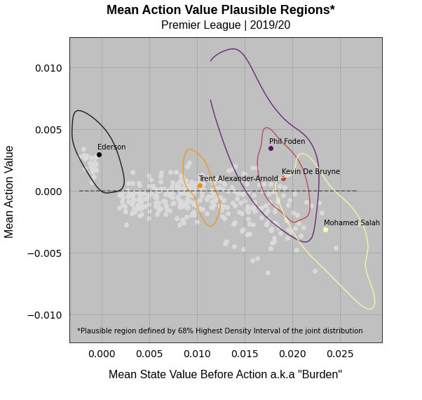
We’ve still got the mean values plotted as a point, but we can now define a plausible region on the plot for each player. The single point model absolutely loves Phil Foden. But our probabilistic version gives us an additional note of caution. It can’t be sure at all really where he should lie on this plot as the plausible region is so large. On the plus side the bulk of this region lies above the zero value dotted line, so we can say with confidence that he is a value adder despite carrying high value burden. Compare this with Kevin De Bruyne, who the model is a lot more confident about, as shown by the much smaller region.
Consider this when looking at your next scatterplot that has modelled variables such as xG and xT axes on Twitter. If you work at a club you should probably be demanding this kind of information from your model supplier if you don’t have it – whether they can give it to you is another story!
Match Timelines
Another staple of the Twittersphere is the rolling match timeline. We’ve seen xG match timelines for a while now and more recently xT has made an appearance. What would a probabilistic action value timeline look like potentially?
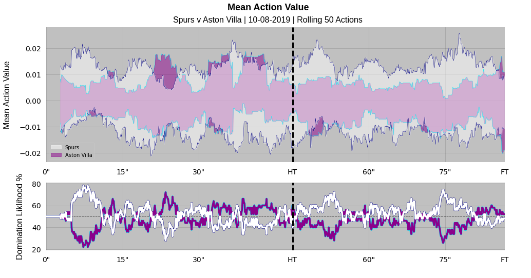
If we take Spurs v Aston Villa early in the 2019/20 Premier League season as an example, you can immediately see a possible downside in interpretation. If we first of all focus on the top plot of the pair, rather than a single line navigating its way across the graph we now have shaded regions. The amount of uncertainty here leads to regions overlapping considerably. As a result it is hard, if not impossible to discern who is actually dominating the match based on the value they are creating.
As a broad concept this kind of chart has the potential to be useful to analysts interested in the underlying value creating process in a match rather than outcomes such as the scoreline or indeed shots taken. The advantage over xT is we can consider the occasions where value was lost, and indeed gained in situations that didn’t result in a direct progression into a dangerous area. But here we see that the uncertainty in the model is swamping visible signal.
One idea to combat this is shown in the bottom of the two plots. Given we have two distributions overlapping at every point in time we can calculate the percent chance that the true value from one team was greater than the other, and then loosely equate that to the concept of “dominance”. We then get a rolling domination index of sorts which is essentially saying “given the information the model saw, there is an x% chance that team A was creating more value than team B at this moment in the game”. Based on a grand sample size of 1 via a BBC match report from the game, it has done a reasonable job of describing the pattern of the game, with a very back and forth first half and completely dominant Spurs in the second half.
Value Sources and Sinks
Something a little bit different now to finish with and to try and hammer home the power of the extra information that a distribution gives you vs a single point estimate.
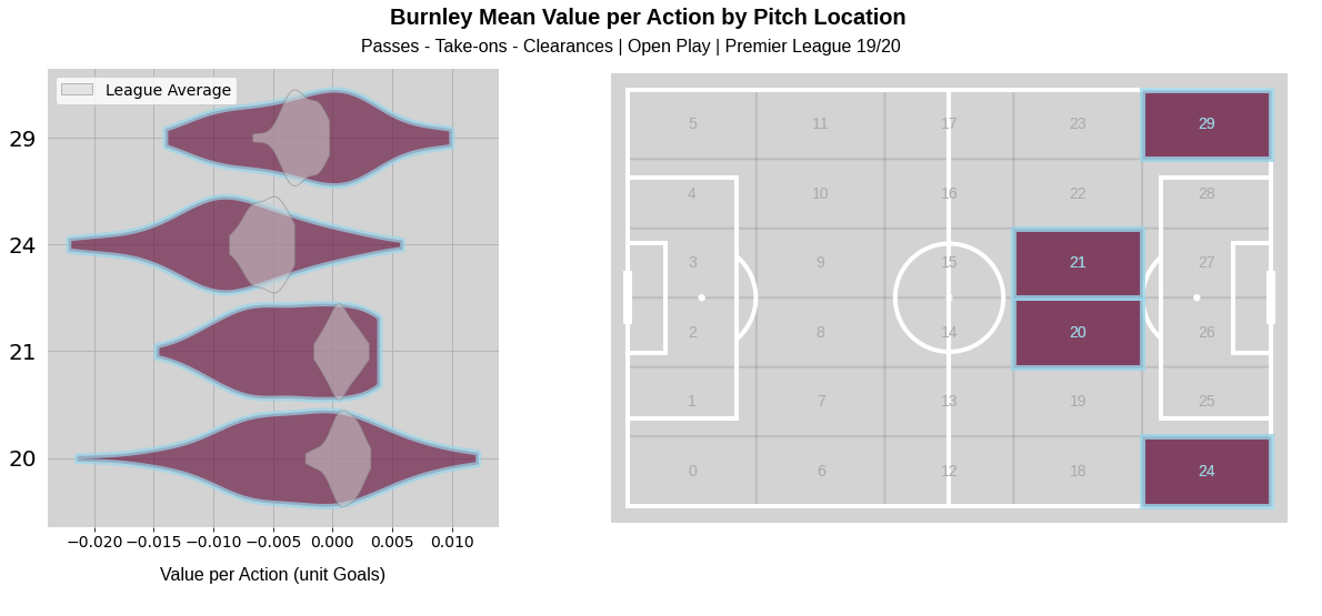
We can look at areas of the pitch for a team and examine whether they generate value from an area or if value gets sucked into a footballing black hole. Let’s take Burnley here, and particularly the central area outside the attacking penalty area you might associate with “zone 14” which I am for some reason denoting “zone 20 and 21”. We know from tactical theory and other works of statistical analysis that this zone can be highly profitable. Indeed the model agrees, with the vast majority of the average Premier League action distribution in this zone gaining value. But it looks like Burnley probably have more trouble doing so in this region. Perhaps if we were playing Burnley next, more focus should be placed on combating opponent possession on the left-hand side, where there is a decent chance they can add value here, maybe more so than league average.
But we get an in-built word of warning as we can see the magnitude of uncertainty is such that they could plausibly be generating positive value in all these areas. Video analysis that would obviously be carried would build up another part of the picture, but now we can actually contribute and potentially challenge existing evidence we’re building up about how a team are likely to play and perform in the future as opposed to producing a single value which would immediately be (probably rightly) trumped by opinion from video analysis.
We can of course divide the pitch however we want here, and look at how opponents generate value vs a team in different areas to evaluate defensive performance.
Conclusion
The key takeaway from all of this would be the more knowledge we know is missing from a model through lack of quantity or context contained within data, the more we know the single value output decreases in usefulness while at the same time increasing the instability of our model.
If there are doubts about the completeness of information being fed into a model, techniques such as those discussed here are almost certainly appropriate and may be essential for use in a real world decision making process.
In addition, many model types report a mean value that minimises overall error, but isn’t anywhere near accurate for individual predictions. With full probabilistic outputs using techniques such as MDNs, although we can’t add extra information into the model we can at least acknowledge that the output could feasibly be a whole range of values. So the player who wrong-foots two defenders with a sideways pass that allows a teammate to drive unopposed towards goal can at least get some credit compared to none or even negative values from a single point model equivalent.
To be clear, adding a quantified measure of model uncertainty doesn’t mean we can start running the game in a spreadsheet or a Python terminal. Informed human judgement (with emphasis on the word ‘informed’) will for the foreseeable future always outperform statistical models overall, all things being equal. But human judgement can and will fail at times, and humans can’t watch all the games. These are part of the reasons why analytics exists after all. So what we do have now is the power to know when to pipe up and challenge traditional video analysis and live scouting and when to keep quiet knowing our model really doesn’t have a clue – which will be often.
As a final thought, it is worth mentioning the cases where we do have high quality and fully contextual data to hand. Are single point value models with tracking data or event data with player freeze frames (as recently announced by StatsBomb) acceptable?
The hope would be that with enough data of this type, the esoteric uncertainty could be reduced significantly. In addition with this extra information, you have a chance at least to achieve mean values that are indistinguishable enough from the true value such that standard binary classification outputs will provide the aleatory uncertainty. I would still say some kind of esoteric uncertainty evaluation e.g. through bagging would always be useful, even if not reported to the end user, just to understand how the model behaves and areas where it struggles to perform optimally.
Acknowledgements
VAEP - Decroos, T., Bransen, L., Van Haaren, J. and Davis, J., 2019, July. Actions speak louder than goals: Valuing player actions in soccer. In Proceedings of the 25th ACM SIGKDD International Conference on Knowledge Discovery & Data Mining (pp. 1851-1861).
Data for VAEP demonstration - StatsBomb

MDN model building - Keras MDN Layer - https://github.com/cpmpercussion/keras-mdn-layer
Pitch plotting - mplsoccer
Pitch plotting debugging - Andy Rowlinson
Additional reference - Sungjoon Choi, Kyungjae Lee, Sungbin Lim, and Songhwai Oh. Uncertainty-aware learning from demonstration using density networks with sampling-free variance modeling. In 2018 IEEE International Conference on Robotics and Automation (ICRA), pages 6915– 6922. IEEE, 2018
