-
A step-by-step guide demonstrating how to generate a finishing ability metric from scratch including confidence interval
-
Typically over/under performance of goal output vs xG is used as an indicator of this ability. This is highly problematic as noise drowns out signal in all but the most extreme abilities or with several seasons’ worth of shots
-
Less common approaches that offer some improvement utilise Bayesian methods. However either the impact of goalkeeper and defender performance is still a component of the output or no attempt at incorporating shot placement and power is made, keeping noise levels high
-
The method presented makes use of a redefined post-shot xG, producing something that is applicable to finishing evaluation - unlike the shot on target only version commonly used to evaluate goalkeepers
Finishing ability is something, along with goalkeeper shot stopping ability, that the public analytics community spends a disproportionate amount of time trying to analyse compared to the actual value it adds to player evaluation.
This is no doubt partly due to the fact that goals scored and conceded by players are telling us exactly what happened, there is no inference or judgement required. It was either a goal or it wasn’t, so there’s (supposedly) no way that bias can creep in to evaluation. Here we have a fast-track route towards evaluating how a player is affecting the outcome of a game handed to us on a plate.
Of course when we put some more consideration into what is driving game outcomes we know that the importance of the final action before a goal is scored or conceded pales in comparison to the many more actions that took place before it both on and off the ball.
But it is not just the motivation that is misguided, it is also the application in many cases. Ability models incorporating goals output are often used in tandem with an expected value, namely xG for finishing and psxG/xG2 for shot stopping. This setup leads to a shot event being treated as a random trial, and as such any differences in ability between professional players is drowned out by the noise of this process unless the ability of the player is truly exceptional or many hundreds (in some cases thousands) of shots are available for a player.
G-xG and psxG-G based ability metrics may have some value as trivia when looking at a player’s career retrospectively, but they should be nowhere near professional analysis. Of course those who evaluate players for a living know that already.
So when it comes to player evaluation, finishing or shot stopping ability should:
-
Only make up one of many traits measured for player evaluation
-
Utilise a calculation method that avoids goals scored/conceded as a differentiator
With that in mind I’ll walk-through a method for deriving a metric of finishing ability over time that is less susceptible to noise than G-xG based methods for the quantities of shots seen in football. Additionally, we can define a confidence interval for values this metric provides. There are of course limitations which will be discussed, but I believe the effort put in here and with the further extensions suggested is proportionate to the value provided.
We’ll be using the fantastic StatsBomb open data set throughout this walk-through. Let’s begin.
Introduction
We’re going to employ strategy a) for improving upon G-xG based metrics which I referred to on Twitter a little while ago. We will keep this metric entirely in the probability domain, so ability will be derived from a change in probability pre-shot vs post-shot. We eliminate all noise stemming from the outcome of processes that are being modelled as random, and all noise is purely as a result of the model components themselves.
We know xG/psxG +/- goals is a low quality metric unless you have at least hundreds shots at your disposal due to the fact you've taken what might be a high quality xG/psxG model and masked it with the outcomes from a set of random trials.
— Charles William (@openGoalCharles) July 24, 2020
A quick thread on some alternatives:
We are therefore going to make use of both xG, and the concept of psxG. To be absolutely clear from the start, psxG here is the same general concept of the well known metric going by the same name that you are probably familiar with for evaluation of goalkeepers. This implementation has marked differences.
psxG, also known as xG2, in current analytics literature is defined as the probability of a shot resulting in a goal given the post- shot characteristics of said shot and also given it is on target. For this reason I am in favour of this metric referring to shots on target in its name in some way, as post-shot expected goals is a much broader concept of which there can be multiple variants measuring different things.
We will be using such a variant in this walk-through, but it will still be referred to as psxG for convenience as it represents post-shot expectation. We are going to develop two models from scratch: an expected goals model, and a post-shot expected goals model that includes all shots. We’ll then use both these models together to infer shooting ability of a small selection of players. We will exclude the data for this selection of players in both the training and testing process and treat it as new data.
xG model
We’re going to keep things simple as much as possible while at the same time trying to maximise the quality of both sub-models. That said the models here will be demonstrated to be of a reasonable quality.
We’ll use a decision tree based model as these are known to perform well in this application and make use of the high performing xgboost algorithm and associated Python library. With this library you can produce high quality models in one line of code and be none the wiser to what is going on under the hood, so I highly recommend some background reading into this incredible piece of technology.
Lets define some model inputs:
-
Shot x location (float)
-
Shot y location (float)
-
Goalkeeper x location (float)
-
Goalkeeper y location (float)
-
Header (boolean)
-
Number of defenders in cone (integer)
The first 4 inputs are pretty self explanatory. Header is simply a true or false value as to whether the shot was a header. The final input is simply the number of defenders, not including the goalkeeper, that are positioned in the cone/triangle created by the points of the shot location, the left post, and right post. There are far better ways to include defender position in a model, such as density or even their x,y co-ordinates, but for this walk-through we will keep things simple.
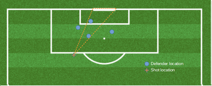
In this case 2 defenders are recorded as being situated within the cone (orange dotted line)
So to describe it in words, our model will predict the probability of a goal based on where the shot was taken from, where the goalkeeper was, whether or not it was a header, and how many defender bodies were in between the ball and the goal.
The positional data of the shot and goalkeeper is relatively straightforward to extract, the only bit of work required is picking out the GK from the shot’s StatsBomb freeze frame. To calculate the number of defenders in the cone comprised of the coordinates of the shot and each of the two goal posts we will make use of the shapely Python package. This package contains functions that allow us to return true or false if a point is inside a shape made up of points we define. All we do is for each shot, run through the each defender (excluding goalkeeper) in the freeze frame and return true or false if their location is in our defined cone. Then we count how many trues we have for the shot.
Taking just these 6 input fields and training on our set of 14,600 shots, we can achieve a log loss of 0.2977 when we test on a set of 6,300 shots that are unseen to the model. This looks like a reasonable figure for this problem based on experience, but as always we have to inspect the calibration curve to ensure our output is representative of true probability.
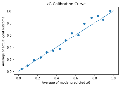
xG model calibration curve - used to inspect alignment between model output and true probability of goal outcome
This looks decent enough to do a job, bearing in mind we’re only using 6 very simple input features. As often seen there his higher variance from implied truth around the higher xG predictions. It is unclear if this is due to a model defect or the smaller number of samples seen at these higher xG values. We’ll deem this model good enough to continue with.
psxG Model
This is probably the more interesting part. psxG is starting to elicit the same reactions from stats enthusiastic public that xG used to all those years ago. As a concept I actually think it gets a bad wrap, as it is mainly it’s misuse in widely shared analysis that causes issue. The thing to remember is that psxG is family of descriptive models. The now well known shot on target variants used to evaluate goalkeepers are often seen as the sole definition of psxG whereas this is actually not the case.
You often see queries on social media within the analytics community about using psxG to measure shooting ability, and this idea is rightly shot down when talking about the SoT variant. Firstly, by stripping out all shots that aren’t on target you lose all data concerning a substantial proportion of a player’s shots. A player could have near perfect shot quality recorded from the 5 shots they took that were on target, but if they took 100 more off target shots which we’ve ignored, what use is the on target data to us for evaluating shooting ability?
Secondly, we have to omit goalkeeper position for SoT psxG. This is because when evaluating a goalkeeper their positioning obviously has a huge bearing on the likelihood of saving a shot. And when their positioning can be deemed to be in their control (a massive challenge to figure out in itself!), we absolutely need to consider it when talking about goalkeeper ability and so must omit it as an input variable to the model.
Flipping this around to evaluating the shooter, we need to include goalkeeper position in the model as the shooter will be making a decision on their target with the goalkeeper position in mind. So we need to evaluate how well they made that decision as part of measuring their ability. Using the SoT variant we can’t do that.
So let’s now define a variant of psxG that is suitable for shooting evaluation. We’ll also keep in mind that we want our psxG model to be simple yet performant and use the same pre-shot input variables as our xG model. More on why the latter is the case later.
Let’s define model inputs:
-
Shot x location (float)
-
Shot y location (float)
-
Goalkeeper x location (float)
-
Goalkeeper y location (float)
-
Number of defenders in cone (integer)
-
Header (boolean)
-
Shot implied ground trajectory (radians - float)
-
Shot implied elevation (radians - float)
-
Shot implied average velocity (m/s - float)
We have added 3 post-shot variables to our pre-shot xG model, increasing the amount of information that will determine the probability of a shot resulting in a goal. A couple of implications become clear straight away. Firstly, a shot which has overall trajectory (both ground and elevation) which suggests it will miss the goal should have a psxG value of zero. Although there is a chance that an off target shot could be deflected back on target mid-flight, the observation we are using for the calculation is the shot’s intercept point with a defender, goalkeeper, or the goal line – and not the trajectory the moment the ball left the player’s boot. Therefore the trajectory value is calculated post-deflection if it happened.
Secondly, a shot that was implied as on target which resulted in a block will have a non-zero psxG value, since there is no guarantee one way or the other if the defender would’ve made the block, unless they are already in contact with the ball when the shot is taken.
There are some obvious sources of noise in this model that can be identified before we’ve even trained it. For example we have a measure of how “busy” the region in front of the shooter is with defenders but we haven’t said where they are located. So while the model will account for the traffic in front of the shot when working it out it’s chances of becoming a goal, there will be times when a shot was always destined to be blocked (i.e. true psxG = 0) which will be given a non-zero value.
Conversely there will be instances where shot has been skilfully aimed away from defenders yet the model will assume it has the average chance of being blocked for that situation when calculating psxG. Not ideal, but log loss and calibration analysis will go some way to telling us if we have enough accuracy to go with.
To calculate ground trajectory we will use the shot location and the location that either a block, off target, wayward, save, or goal event was recorded. Pretty standard stuff. For velocity we will use the distance the ball travelled during the shot event and the recorded duration to calculate average velocity. This is another clear source of model noise since the accuracy of the calculated velocity can be called into question. Basic inspection shows of some of the values coming out of the basic v = s/t calculation are clearly wrong so we’ll do a bit of (very) basic cleaning to reduce the effect of the worst offenders.
Average velocity values will therefore be clipped at 50 m/s so that clearly nonsensical values will be have their velocity noted as a very high value but within the bounds of human feasibility.
For calculating elevation we have to be a bit more creative as we have some missing data to deal with. Elevation can be calculated by taking the angle from ground* to the point on the z-axis the shot event ended. The problem is there is no recorded value for blocked or wayward shots, so we don’t know the elevation for these shot types. We can’t simply omit them from the set, so we need to do some imputation - replacing the missing data with substitute values.
Interestingly, xgboost – our decision tree model Python package of choice here – can accept missing values as an input. This is however undesirable for us as we don’t want the model to work out that all shots that have a missing elevation value will never result in a goal, as the lack of end z location for these shots is just a choice made by StatsBomb and not a feature of the system we are modelling.
Instead we will give these shots an elevation sampled from the distribution of all of the other shots that have a recorded value. We’ll view this distribution first, and note that it has some complexity so we’ll use a non-parametric method to fit it, namely kernel density estimation (KDE). We’ll then randomly sample from this distribution for each missing value.
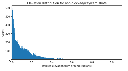
Distribution of implied elevation angle from ground of shots that were not blocked or wayward. This is not generated by an easily identifiable function, so KDE will be used to model it and take new samples from it
Now the model cannot distinguish whether a shot will be blocked, and hence will have zero psxG, based purely on it’s elevation. As a result some shots that were heading over that were blocked may be given an on-target elevation. So we’ve essentially said elevation has no bearing on the chances of a shot being blocked which is clearly false, but this situation is better than the model knowing a shot will have psxG = 0 due to shortcomings in labelling we have in our data set.
Let’s now train the model using the same train and test data we used for the xG model via the same random seed and take a look at the log loss and calibration curve. Encouragingly our post-shot input data with known sources of noise has added significant predictive power. Log loss is now 0.2479 and we have improved calibration. This improvement is what we would have hoped for. With post shot information we can now make a more refined estimate of the probability a shot will result in a goal.
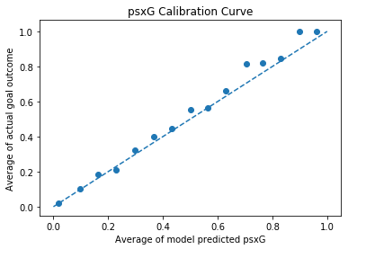
psxG model calibration curve - visually we can see closer alignment to the 1:1 target line (blue dashed) compared to the xG model
To check that the elevation input we tinkered with was actually adding value to model, we can train it again without elevation as an input. The log loss is now considerably lower at 0.2824. So we can be confident that we have increased performance whilst not letting the missing elevation data damage the integrity of the model.
* all shots in the data set used have shot impact height set to ground by default. From 01/08/2020 there is now shot impact height data available for shots from StatsBomb, which if included in the models would likely increase the quality of both xG and psxG outputs.
Putting it all together
Let’s now return to our small set of shots we stripped out at the very beginning which belong to some evaluation players. We can assign an xG value and a psxG value for each of their shots. We therefore have a measure of the probability of scoring at the moment they elected to shoot based on the post-shot characteristics of shots taken by all players which we call xG. We also have a measure of what the probability of scoring was the split second after the shot was taken based purely on the post-shot characteristics that were the result of the shooter under evaluation which we call psxG. Therefore it is reasonable to assume that any difference in post vs pre shot probability given our model definitions is solely down to the player who took the shot.
In essence we are saying that psxG – xG, or probability difference, is a result of variables under the control of the player under evaluation only and therefore can be used as proxy to measure their shooting ability.
As touched upon earlier, by having a set of common inputs and identical model structure and subtracting one model output from the other, we can eliminate some non-zero mean error, or bias, that stemmed from those common inputs which is advantageous. A clear negative of this approach is that we are using 2 separate models which have their own noise (both the biases we couldn’t eliminate and the zero mean noise) contributions.
We know using G-xG as a measure of shooting ability has a large noise component stemming from the fact we are modelling the shot as the outcome of a random trial, but at least there is only one model for additional noise to originate from. Does this approach using two models give us a less noisy, and therefore more predictive value than the G-xG approach? Let’s take a look for one of our evaluation players: Alexis Sánchez.
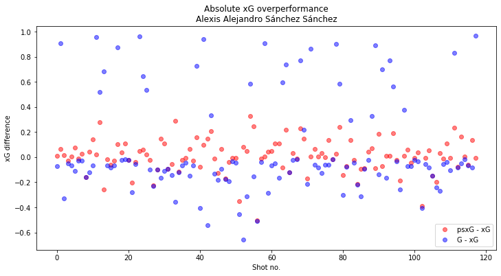
We can immediately see the variance between each measurement, or shot taken, is considerably lower with the psxG method compared to the goals method. We would of course expect this since psxG is another probability value whilst G is a 0,1 outcome. But how confident can we be that our measurement is actually reflecting ground truth ability? With G-xG at least we have data about what actually happened so we know there is ability signal in there somewhere (the problem being in the vast majority of cases we can’t see it due to the magnitude of noise). We don’t know if there is signal for the psxG-xG case as the metric is based purely off of two models.
We know the models are roughly in the right place from our log loss and calibration performance. If we can isolate where the uncertainty in our model comes from then we can attach a level of confidence to the value that our metric outputs, rather than accepting a single value with blind faith. Two key categories of noise that will be generated in a model such as this are input measurement error and model error. Accounting for the former is beyond the scope of this article, but this noise stems from the fact that the values that are input into the model are different from their true value. This could originate from inaccuracies in measurement from technological shortcomings, human error, or rounding values up/down.
The noise category we will cover and account for with our finishing ability metric is the noise that arises from the within the model itself. All models are approximations of a system in one way or another. This may be due to information about the system being missing or relationships between system variables being expressed in a simplified manner. In this case we have plenty of missing information about the situation the shot was taken in and the attributes of the shot after it was taken that could be used to determine xG and psxG. We are also expressing relationships between variables as a decision tree with shots that are deemed similar enough grouped together. So how does the interplay between these modelling shortcomings affect the values we get out of our model?
One way of evaluating this is to train the model multiple times under different conditions and inspect the distribution of the range of outputs we get for a common test input. In a perfect model we would expect to get the same output for any given input, but in reality the output will vary between models trained under different conditions. For each run of the training process the effect of missing information will vary and the model will have to generate a different idea of how input variables relate to each other. By evaluating the range of values we get for our predictions produced by the different training runs we can gauge how much this variability matters. This will then serve as a confidence interval based on whatever level of confidence we choose.
So let’s train both the xG and psxG models 1000 times, each time generating our train and test sets from a new random seed. We can then take one of our evaluation players’ shots and run it through each of 1000 models to give 1000 xG, psxG pairs per shot.
We then calculate relative overperformance, psxG-xG / xG, for each pair. It is appreciated that there will be performance variability reflected in our output on top of latent ability and that this ability can vary over time. We therefore have a time series on our hands, so we’ll calculate a rolling average for our overperformance measure. This value can be set to anything the analyst wants, with the trade-off being lag/responsiveness vs variance. We’ll choose 30 shots here.
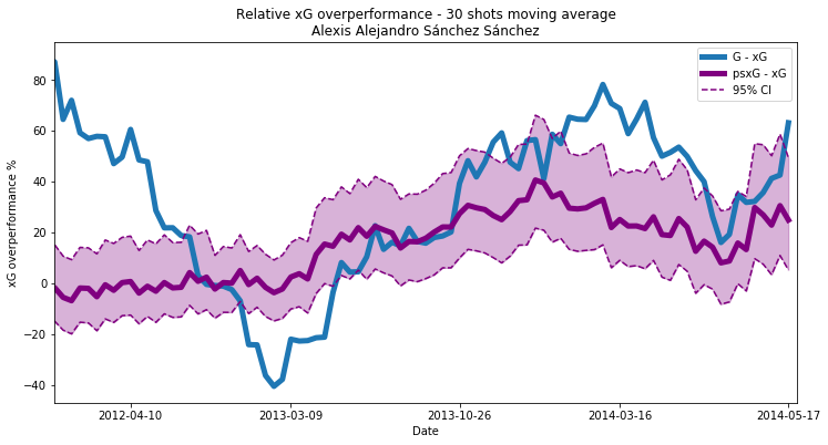
Looking at the over-performance time-series for Alexis Sánchez within the StatsBomb data set we can see his actual goal output vs expected (blue line) zig-zagged quite dramatically over a two year period. At the start of 2011/12 he over-peformed by over 80% initially, but then a dramatic decline commenced culminating in an under-performance of -40% by March 2013. Our baseline metric (purple line) shows it was factors outside of his control that was leading to this trend, and he was in fact pretty much always over-performing vs expectation from April 2012 to May 2014.
Moving on to the second key feature of our metric which is the shaded region representing the 95% confidence interval. The dotted lines are the 2.5% and 97.5% percentiles of the rolled averages calculated from the set of 1000 model outputs we generated. One thing to appreciate from the start is that even with many thousands of data points at your disposal to train a model, the output often will be sensitive to the data used to train it – this is not a phenomenon unique to this implementation.
For Alexis Sánchez, our model - for which we know both sub-models have decent predictive power and are well calibrated to outcomes - has identifiable periods where he is over-performing average with a 97.5% confidence (as 97.5% of the distribution is above average) with a 30 shot window. The psxG based model also appears to be an attenuated version of the G-xG based model from March 2013 onward, which isn’t necessarily unexpected since it just means the variables outside of Alexis Sánchez’s control played out roughly as expected.
As mentioned, there is more noise to add stemming from the accuracy of our input data which would widen our interval, but of course the same goes for the G-xG based model. So it looks at least as though we may have a better chance of identifying ability signal than the G-xG based model, which is what it was all about.
The plots for the other 2 players chosen for evaluation (out of a very small number of players who have a reasonable number of shots over reasonable length time period) are shown below. Clearly we need more than 3 players’ worth of data to validate this method properly, but we don’t have the means with the data available.
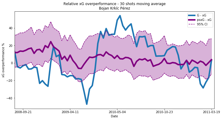
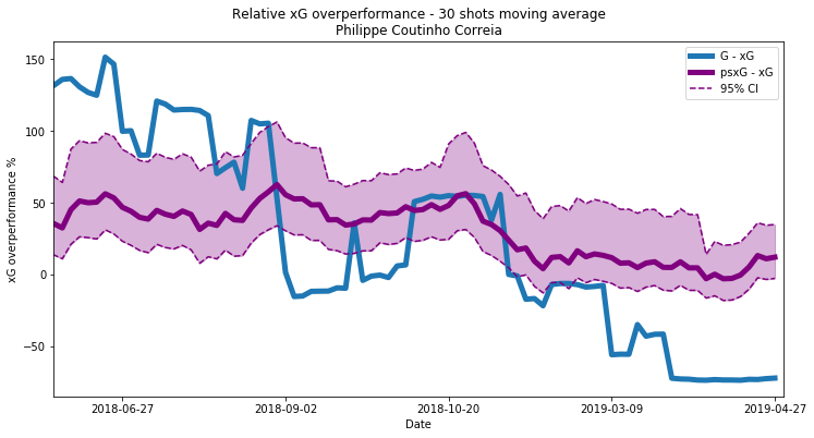
A key thing to note is that these values are not strictly directly comparable between players, although you can probably get away with it under most circumstances and with wider averaging windows. While we have controlled for varying xG distributions of players by using a relative metric value, the scope to over or under perform as a percentage of xG is still determined by the baseline xG value. For exaple a player taking 30 shots with xG = 0.9 can only over-perform by a maximum of 11.1%, whereas a player taking 30 shots with xG = 0.1 could theoretically over-perform by up to 900%. So as always an extra step is required when using a metric such as this in taking care that any comparisons between players are valid.
Wrapping up
There is a decent foundation to build upon here as a higher quality alternative to G-xG for measuring finishing ability. Even with evaluation on just three players, the metric looks relatively stable which we would expect when measuring ability, with trends occurring over longer time frames which represent genuine changes. There are still clear flaws however. The first things I would do to take this method further would be:
-
Train and evaluate the model on a data set with high quality scope. So not with 30% women’s, 70% men’s as we’ve used here. And certainly not 10% Lionel Messi!
-
Incorporate the StatsBomb shot action height input into the model and investigate adding further input features both for xG and psxG sub-models. A categorical representing bend angle from straight-line springs to mind as a post-shot variable that could have an affect of goal probability.
-
Investigate other model architectures and hyperparamter optimisation. This xgboost model has only undergone only very basic hyperparameter tuning.
-
Look to quantify error magnitude for all input variables. Then evaluate the sensitivity of the model output to deviations of input variables by these magnitudes.
As a final note it is worth mentioning that there are other methods for trying to identify finishing ability. In my view the two best pieces on the subject are by Marek Kwiatkowski and Laurie Shaw. Both of these methods utilise Bayesian techniques, but perhaps Marek’s is slightly more innovative in that an attempt is made to incorporate the shot taker as an input into the xG model.
Another way would be to measure how close a shot was to resulting in a goal using a smooth reward function as opposed to the all or nothing approach of familiar approaches. That way a shot that narrowly misses at least gets some credit, just like a weak, very savable shot that is on target does. I haven’t seen any public work that is based on this concept, but I may visit this method on this site at some point in the future.
Acknowledgements
This work has been made possible due to the generosity of StatsBomb and their open data initiative.
